Python Package

In most cases, moDiNA can be conveniently used as a standalone Python package. For users interested in systematically comparing results across multiple moDiNA configurations, a dedicated Nextflow pipeline is provided.

Installation

moDiNA can be installed using Conda, Docker of from source. If you face any issues, feel free to open an issue on GitHub.

With Conda

Currently, the moDiNA package is only available on GitHub. moDiNA requires Python version 3.11.

It is recommended to install moDiNA in a clean conda (Miniconda) environment. We suggest using mamba, a faster drop-in replacement for conda that improves dependency resolution. Mamba is automatically installed when using Miniforge.

First, follow the installation instructions for your operating system. Then create and activate a new environment:

mamba create -n modina_env python=3.11
mamba activate modina_env

Next, install the package:

pip install git+https://github.com/DyHealthNet/moDiNA.git

With Docker

moDiNA is available as Docker image.

Pull the image:

docker pull ghrc.io/dyhealthnet/modina:latest

Run the image:

docker run -it ghrc.io/dyhealthnet/modina:latest

From Source

To install moDiNA from source, clone the repository and install the package using pip:

git clone https://github.com/DyHealthNet/moDiNA.git
pip install -e .

Data Input

Real-World Data

To run moDiNA on your own data, you need two pandas DataFrames containing the sample data from two biological conditions (e.g. healthy and diseased). Each row represents a sample, while each column corresponds to a variable.

Both DataFrames must contain the same set of variables. However, they may differ in the number of samples, as samples are generally assumed to be independent.

The data type of each variable must be specified in a metadata file containing two columns: label and type. Supported variable types are continuous, binary, nominal, and ordinal. Categorical variables must be encoded as numerical values.

The tables below show an example of a context DataFrame and the corresponding metadata file.

Context Data

	Protein_A	Protein_B	Gender	Disease_Stage	Ethnicity
S1	2.31	5.12	0	1	2
S2	3.04	4.87	1	2	0
S3	2.76	5.33	0	3	1
S4	3.18	4.95	1	2	2

Metadata

label	type
Protein_A	continuous
Protein_B	continuous
Gender	binary
Disease_Stage	ordinal
Ethnicity	nominal

Simulated Data

Alternatively, the simulate_copula function allows you to generate two synthetic biological contexts with continuous, binary, and ordinal categorical variables, using Gaussian copula sampling. The occurrence and magnitude of differential effects can be controlled via the input parameters, allowing users to introduce both differential abundance and differential associations between variables. This approach is particularly useful for benchmarking moDiNA under controlled conditions.

Parameters:

• name1, name2: Names of the two biological contexts.

• n_cont, n_bi, n_cat: Number of continuous, binary and ordinal variables per context, respectively.

• n_samples: Number of samples per context.

• n_shift_*: Number of variables with an artificial mean shift. Replace * with the variable type, e.g., n_shift_cont, n_shift_bi, n_shift_cat.

• n_corr_*: Number of variable pairs with a correlation difference. * represents the variable type combinations, e.g., n_corr_cont_cont, n_corr_bi_cat, etc.

• n_both_*: Number of variable pairs with both a mean shift and a correlation difference. * represents variable type combinations as above.

• shift: Approximate magnitude of the mean shift measured in standard deviations (differential abundance). Defaults to 0.5.

• corr: Approximate magnitude of the correlation difference measured as correlation coefficient between 0 and 1 (differential association). Defaults to 0.7.

• path: Optional path to save simulated contexts, metadata, and ground truth.

Returns:

A tuple (context1, context2, meta, ground_truth):

• context1: pandas DataFrame of the first simulated context.

• context2: pandas DataFrame of the second simulated context.

• meta: pandas DataFrame containing the data type for each variable.

• ground_truth: Tuple of three lists specifying the nodes with differential effects:

  • nodes with mean shifts,

  • nodes with correlation differences,

  • nodes with both mean shifts and correlation differences.

Example:

from modina.context_simulation import simulate_copula

context1, context2, meta, ground_truth = simulate_copula(
    n_cont=30,
    n_bi=20,
    n_cat=10,
    n_samples=200,
    n_shift_cont=5,
    n_corr_bi_cat=2,
    n_both_cont_cat=2,
    shift=0.8,
    corr=0.6
)

Differential Network Analysis

The recommended way to use moDiNA is to execute the complete analysis pipeline via the diffnet_analysis() function. It performs context network inference, edge filtering, differential network construction, and ranking of nodes and edges. All configuration options can be specified directly through the function arguments.

Parameters:

• context1, context2: pandas DataFrames containing the observed data for the two contexts (rows: samples, columns: variables).

• meta_file: pandas DataFrame specifying the variable metadata. Must contain the columns label and type describing each variable and its data type.

• edge_metric: Edge-level metric used to compute the differential network. Options include 'pre-P', 'post-P', 'pre-E', 'post-E', 'pre-PE', 'post-PE', 'pre-LS', 'post-LS', 'int-IS'.

• node_metric: Node-level metric used to compute the differential network. Options include 'DC-P', 'DC-E', 'WDC-P', 'WDC-E', 'PRC-P', 'STC'.

• ranking_alg: Ranking algorithm applied to the differential network. Options include 'PageRank+', 'PageRank', 'absDimontRank', 'DimontRank', 'direct_node' and 'direct_edge'. Defaults to 'PageRank+'.

• filter_method: Optional filtering method applied before constructing the differential network. Options include 'quantile', 'degree', 'density'. Per default, no filtering is performed.

• filter_param: Parameter controlling the filtering strength.

• filter_metric: Edge metric used for filtering.

• filter_rule: Rule used to integrate the two networks during filtering. Options include 'union' and 'zero'.

• max_path_length: Maximum path length considered when computing integrated interaction scores. Defaults to 2.

• test_type: Statistical test used for association score calculation. Options include 'parametric' and 'nonparametric'. Defaults to 'nonparametric'.

• nan_value: Numerical value used to replace missing values in the context data. If None, an error is raised when missing values are present.

• correction: Multiple testing correction method. Options include 'bh' (Benjamini-Hochberg) or 'by' (Benjamini–Yekutieli). Defaults to 'bh'.

• num_workers: Number of parallel workers used during score computation. Defaults to 1.

• project_path: Optional directory where intermediate results and output files will be stored.

• name1, name2: Names of the two contexts used for labeling and output file generation.

Tip

Based on an extensive benchmark analysis performed on simulated data, we recommend the following pipeline configuration:

• Edge Metric: pre-LS

• Node Metric: STC

• Ranking Algorithm: PageRank+

Returns:

A tuple (ranking, rankings_per_type, edges_diff, nodes_diff, config):

• ranking: List containing the overall ranking of nodes or edges based on the selected ranking algorithm.

• rankings_per_type: Dictionary containing rankings stratified by variable type. Type-specific rankings can be accessed using the keys 'cont', 'cat', and 'bi'.

• edges_diff: pandas DataFrame containing the differential edge scores.

• nodes_diff: pandas DataFrame containing the differential node scores.

• config: Dictionary containing the configuration parameters used in the analysis.

Example:

from modina.pipeline import diffnet_analysis

ranking, rankings_per_type, edges_diff, nodes_diff, config = diffnet_analysis(
    context1=context1,
    context2=context2,
    meta_file=meta,
    edge_metric='pre-LS',
    node_metric='STC',
    ranking_alg='PageRank+',
    filter_method='quantile',
    filter_param=0.5,
    filter_metric='pre-P',
    filter_rule='zero'
)

Note

If a specific step of the pipeline needs to be recomputed or adjusted, it may be useful to execute the analysis steps separately instead of rerunning the entire pipeline. The individual steps are descibed below.

Context Network Inference

To infer context-specific networks, the compute_context_scores function calculates association scores for a single biological context. Parametric (P) or non-parametric (NP) data type-specific tests and multiple testing correction is performed using NApy, which efficiently computes pairwise statistical tests and provides enhanced support for missing data. Missing values must be encoded as a common numerical value. The resulting effect sizes and p-values quantify the strength of the relationships between variables and are used to construct a context-specific network, where variables are represented as nodes and association scores as weighted edges. The table below provides an overview of all implemented statistical tests.

Test	Effect Size	Range	Data	Type
Pearson	r	[-1, 1]	Cont–Cont	P
Spearman	ρ	[-1, 1]	Cont–Cont, Cont–Ord, Ord–Ord	NP
t-test	Cohen’s d	(-∞, ∞)	Cont–Bin	P
Mann–Whitney U	Cohen’s d	(-∞, ∞)	Cont–Bin, Bin–Ord	NP
ANOVA	Partial η²	[0, 1]	Cont–Nom	P
Kruskal–Wallis	η²	[0, 1]	Cont–Nom, Ord–Nom	NP
χ²-test	Cramer’s V	[0, 1]	Bin–Bin, Bin–Nom, Nom–Nom	P, NP

Parameters:

• context_data: pandas DataFrame containing the observed data (rows: samples, columns: variables).

• meta_file: pandas DataFrame specifying the variable metadata. Must contain the columns label and type describing each variable and its data type.

• test_type: Statistical tests used for network inference. Options include 'parametric' and 'nonparametric'. Defaults to 'nonparametric'.

• correction: Multiple testing correction method. Options include 'bh' (Benjamini-Hochberg) or 'by' (Benjamini–Yekutieli). Defaults to 'bh'.

• num_workers: Number of parallel workers for computation. Defaults to 1.

• path: Optional file path to save the computed scores as a CSV file. Defaults to None.

• nan_value: Numerical value used to replace missing values in the context data. If None, an error is raised when missing values are present.

Returns:

A pandas DataFrame containing the computed association scores for all variable pairs.

Example:

from modina.context_net_inference import compute_context_scores

scores = compute_context_scores(
    context_data=context1,
    meta_file=meta,
    test_type='nonparametric',
    correction='bh',
    num_workers=4,
    path='context1_scores.csv',
    nan_value=-999
)

Edge Filtering

The statistical network inference step produces fully connected networks, where every pair of variables is linked by an edge. To reduce network complexity, insignificant edges with large p-values or small effect sizes can be removed using the filter function.

Three different filtering methods are available, all following the same basic principle: edges are first ordered according to their association scores and then thresholded to achieve a desired network characteristic. The quantile method retains only the strongest fraction of edges, the degree method reduces the network to a specified average node degree, and the density method enforces a predefined network density by keeping only a certain percentage of all possible edges.

After filtering, there are two alternative rules for integrating the two networks. The union rule retains all edges that are present in either network, preserving their original association scores. This approach can recover edges that were eliminated in one network. However, the resulting context-specific networks remain structurally identical. For edge metrics such as DC-P or DC-E, which rely solely on network topology, it is therefore recommended to use the zero rule instead. Under the zero rule, removed edges are treated as missing and will be assigned insignificant p-values of 1.0 and effect sizes of 0.0 in downstream calculations.

Parameters:

• scores1, scores2: pandas DataFrames containing the statistical association scores for Context 1 and Context 2.

• context1, context2: pandas DataFrames with the raw context data for Context 1 and Context 2.

• filter_method: Filtering method to apply. Options include 'quantile', 'degree', or 'density'. Defaults to None (no filtering).

• filter_param: Parameter controlling the strength or threshold of the filtering method.

• filter_metric: Edge metric used as the basis for filtering. Options include the adjusted p-value (use 'pre-P') or the Z-score-normalized effect size (use 'pre-E').

• filter_rule: Rule used to integrate the two networks during filtering. Options include 'union' and 'zero' .

• path: Optional path to save the filtered scores and context data as CSV files. Defaults to None.

Warning

Currently, it is not recommended to use pre-E as a filter metric. Ordering and thresholding Z-score-normalized effect sizes can inadvertently remove highly important edges with large negative effect sizes. This issue will be addressed in an upcoming update. In the meantime, please use pre-P instead.

Returns:

A tuple (scores1_filtered, scores2_filtered, context1_filtered, context2_filtered):

• scores1_filtered, scores2_filtered: pandas DataFrames containing the filtered association scores for each context.

• context1_filtered, context2_filtered: pandas DataFrames containing the raw context data for all variables that remain connected by at least one edge in the filtered networks.

Examples:

from modina.edge_filtering import filter

# Quantile filtering
scores1_filtered, scores2_filtered, context1_filtered, context2_filtered = filter(
    scores1=scores1,
    scores2=scores2,
    context1=context1,
    context2=context2,
    filter_method='quantile',
    filter_param=0.05,
    filter_metric='pre-P',
    filter_rule='union'
)

# Degree filtering
scores1_filtered, scores2_filtered, context1_filtered, context2_filtered = filter(
    scores1=scores1,
    scores2=scores2,
    context1=context1,
    context2=context2,
    filter_method='degree',
    filter_param=5,
    filter_metric='pre-P',
    filter_rule='zero'
)

# Density filtering
scores1_filtered, scores2_filtered, context1_filtered, context2_filtered = filter(
    scores1=scores1,
    scores2=scores2,
    context1=context1,
    context2=context2,
    filter_method='density',
    filter_param=0.8,
    filter_metric='pre-E',
    filter_rule='zero'
)

Note

Edge filtering can substantially reduce the runtime of moDiNA for large datasets. It is especially recommended when using the computationally heavy int-IS edge metric to construct the differential network.

Differential Network Construction

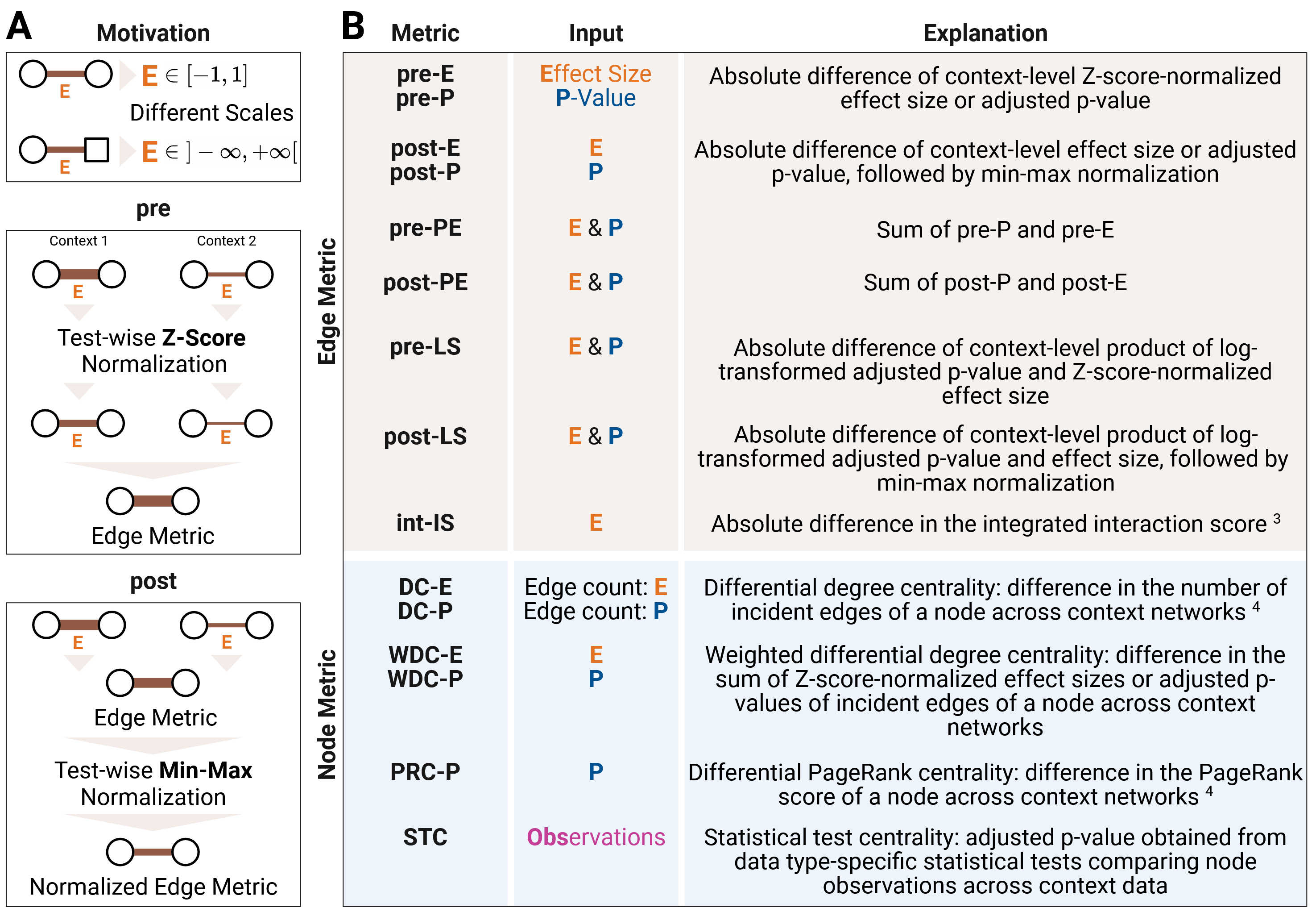
Figure 1: (A) Effect size normalization and (B) definition of differential edge and node metrics. Created with BioRender.com.

Two context-specific networks are aggregated into a differential network using a variety of node- and edge-level metrics provided in the compute_diff_network function. Since effect sizes obtained from data type-specific statistical tests are located on different scales, rescaling is required to make them comparable across data types. This can be achieved either through Z-score normalization, which is used in pre metrics, or through min–max normalization, which is used in post metrics.

Parameters:

• scores1, scores2: pandas DataFrames containing the statistical association scores of the two context-specific networks.

• context1, context2: pandas DataFrames containing the observed data for the two contexts (rows: samples, columns: variables).

• edge_metric: Edge-level metric used to compute the differential network. Options include 'pre-P', 'post-P', 'pre-E', 'post-E', 'pre-PE', 'post-PE', 'pre-LS', 'post-LS', 'int-IS'.

• node_metric: Node-level metric used to compute the differential network. Options include 'DC-P', 'DC-E', 'WDC-P', 'WDC-E', 'PRC-P', 'STC'.

• max_path_length: Maximum length of paths to consider in the computation of integrated interaction scores. Defaults to 2.

• nan_value: Numerical value used to replace missing values in the context data. If None, an error is raised when missing values are present.

• correction: Multiple testing correction method. Options include 'bh' (Benjamini-Hochberg) or 'by' (Benjamini–Yekutieli). Defaults to 'bh'.

• path: Optional directory where the computed differential scores will be saved.

• format: Output format used when saving the differential network. Options include 'csv' and 'graphml'. Defaults to 'csv'.

• meta_file: pandas DataFrame containing metadata about the variables. Must include the columns label and type. Required when using the STC node metric.

• test_type: Statistical test used for continuous nodes in the STC metric. Options include 'parametric' and 'nonparametric'. Defaults to 'nonparametric'.

Returns:

A tuple (edges_diff, nodes_diff):

• edges_diff: pandas DataFrame containing the computed differential edge scores.

• nodes_diff: pandas DataFrame containing the computed differential node scores.

Example:

from modina.diff_network import compute_diff_network

edges_diff, nodes_diff = compute_diff_network(
    scores1=scores_context1,
    scores2=scores_context2,
    context1=data_context1,
    context2=data_context2,
    edge_metric='pre-LS',
    node_metric='STC',
    test_type='nonparametric',
    meta_file=meta
)

Ranking

The final step in differential network analysis with moDiNA is to rank nodes or edges according to their differential activity using the compute_ranking function. Several ranking algorithms are available, which differ in the type of evidence they incorporate. In particular, algorithms may use differential edge and/or node scores, and may account for the directionality of differential effects. The table below summarizes the implemented ranking methods and their required inputs.

Ranking Algorithm	Input			Output
	Edges	Nodes	Direction
DimontRank	✓		✓	node ranking
absDimontRank	✓			node ranking
PageRank	✓			node ranking
PageRank+	✓	✓		node ranking
direct_node		✓		node ranking
direct_edge	✓			edge ranking

Parameters:

• nodes_diff: pandas DataFrame containing differential node scores.

• edges_diff: pandas DataFrame containing differential edge scores.

• ranking_alg: Ranking algorithm to compute. Options include 'PageRank+', 'PageRank', 'absDimontRank', 'DimontRank', 'direct_node' and 'direct_edge'.

• meta_file: Optional pandas DataFrame specifying node metadata (columns label and type), used to generate type-specific rankings.

• path: Optional file path to save the resulting ranking as a CSV file.

Returns:

A tuple (ranks, rank_dict):

• ranks: List containing the ranked nodes (or edges for direct_edge), sorted in descending order.

• rank_dict: Dictionary containing rankings per data type:

  • 'cont': Continuous variables

  • 'ord': Ordinal variables

  • 'nom': Nominal variables

  • 'bi': Binary variables

Example:

from ranking import compute_ranking

# Personalized PageRank
rankings, rank_dict = compute_ranking(
    nodes_diff=nodes_diff,
    edges_diff=edges_diff,
    ranking_alg='PageRank+',
    meta_file=meta
)